Statistical Analysis

This notebook contains routines for analyzing the output of keypoint-MoSeq.

Note

The interactive widgets require jupyterlab launched from the keypoint_moseq environment. They will not work properly in jupyter notebook.

Setup

We assume you have already have keypoint-MoSeq outputs that are organized as follows.

<project_dir>/               ** current working directory
└── <model_name>/            ** model directory
    ├── results.h5           ** model results
    └── grid_movies/         ** [Optional] grid movies folder

Use the code below to enter in your project directory and model name.

import keypoint_moseq as kpms

project_dir='path/to/project' # the full path to the project directory
model_name='model_name' # name of model to analyze (e.g. something like `2023_05_23-15_19_03`)

Assign Groups

The goal of this step is to assign group labels (such as “mutant” or “wildtype”) to each recording. These labels are important later for performing group-wise comparisons.

• The code below creates a table called {project_dir}/index.csv and launches a widget for editing the table. To use the widget:

  • Click cells in the “group” column and enter new group labels.

  • Hit Save group info when you’re done.

• If the widget doesn’t appear, you also edit the table directly in Excel or LibreOffice Calc.

kpms.interactive_group_setting(project_dir, model_name)

Generate dataframes

Generate a pandas dataframe called moseq_df that contains syllable labels and kinematic information for each frame across all the recording sessions.

moseq_df = kpms.compute_moseq_df(project_dir, model_name, smooth_heading=True) 
moseq_df

	name	centroid_x	centroid_y	heading	angular_velocity	velocity_px_s	syllable	frame_index	group	onset
0	21_11_8_one_mouse.top.irDLC_resnet50_moseq_exa...	245.691668	210.796020	-1.217558	0.000000	0.000000	7	0	mutant	True
1	21_11_8_one_mouse.top.irDLC_resnet50_moseq_exa...	246.797705	208.926666	-1.217558	-0.079308	65.161529	7	1	mutant	False
2	21_11_8_one_mouse.top.irDLC_resnet50_moseq_exa...	246.880092	208.750297	-1.227725	-0.160751	5.839875	7	2	mutant	False
3	21_11_8_one_mouse.top.irDLC_resnet50_moseq_exa...	247.338747	206.761270	-1.240335	-0.246197	61.236711	7	3	mutant	False
4	21_11_8_one_mouse.top.irDLC_resnet50_moseq_exa...	248.073132	205.021514	-1.240335	-0.336099	56.652130	7	4	mutant	False
...	...	...	...	...	...	...	...	...	...	...
643906	22_27_04_cage4_mouse2_0.top.irDLC_resnet50_mos...	217.514933	196.355583	0.193480	-0.618441	565.377392	12	53618	default	False
643907	22_27_04_cage4_mouse2_0.top.irDLC_resnet50_mos...	202.928966	183.149695	0.086206	-0.318911	590.280706	12	53619	default	False
643908	22_27_04_cage4_mouse2_0.top.irDLC_resnet50_mos...	187.950492	169.656667	0.193808	-0.126241	604.793226	12	53620	default	False
643909	22_27_04_cage4_mouse2_0.top.irDLC_resnet50_mos...	173.977080	155.679578	0.302726	-0.026824	592.919672	12	53621	default	False
643910	22_27_04_cage4_mouse2_0.top.irDLC_resnet50_mos...	158.353112	143.198606	0.136897	0.004577	599.912268	12	53622	default	False

643911 rows × 10 columns

Next generate a dataframe called stats_df that contains summary statistics for each syllable in each recording session, such as its usage frequency and its distribution of kinematic parameters.

stats_df = kpms.compute_stats_df(
    project_dir,
    model_name,
    moseq_df, 
    min_frequency=0.005,       # threshold frequency for including a syllable in the dataframe
    groupby=['group', 'name'], # column(s) to group the dataframe by
    fps=30)                    # frame rate of the video from which keypoints were inferred

stats_df

	group	name	syllable	heading_mean	heading_std	heading_min	heading_max	angular_velocity_mean	angular_velocity_std	angular_velocity_min	angular_velocity_max	velocity_px_s_mean	velocity_px_s_std	velocity_px_s_min	velocity_px_s_max	frequency	duration
0	default	21_12_10_def6a_1_1.top.irDLC_resnet50_moseq_ex...	0	-0.185726	1.675327	-3.141268	3.141216	0.006244	5.969984	-188.391070	188.423102	23.873621	18.251097	0.052929	250.661913	0.193452	1.278718
1	default	21_12_10_def6a_1_1.top.irDLC_resnet50_moseq_ex...	1	-0.186075	1.545966	-3.138770	3.141024	-0.047082	9.326394	-188.077053	3.634033	39.028218	31.174287	0.688662	216.440283	0.113839	0.884532
2	default	21_12_10_def6a_1_1.top.irDLC_resnet50_moseq_ex...	2	-0.270518	1.744452	-3.141173	3.140562	-0.237998	12.575613	-187.851585	188.203382	61.339926	45.208260	0.699143	249.923269	0.130208	0.846095
3	default	21_12_10_def6a_1_1.top.irDLC_resnet50_moseq_ex...	3	0.300797	1.392815	-3.139225	3.140805	-0.005278	10.043521	-188.285953	188.290531	35.085909	27.308359	0.488694	234.898832	0.112351	1.552759
4	default	21_12_10_def6a_1_1.top.irDLC_resnet50_moseq_ex...	4	0.004180	1.850509	-3.136158	3.138170	0.292483	13.734939	-188.161345	188.074944	38.752501	31.086649	0.536752	204.338343	0.068452	1.219203
...	...	...	...	...	...	...	...	...	...	...	...	...	...	...	...	...	...
163	mutant	22_04_26_cage4_1_1.top.irDLC_resnet50_moseq_ex...	12	-0.083118	2.002411	-3.127063	3.121900	1.286797	16.501619	-11.525765	186.041027	54.491124	35.084645	1.652698	219.963610	0.020379	0.280460
164	mutant	22_04_26_cage4_1_1.top.irDLC_resnet50_moseq_ex...	13	-0.460300	1.651639	-2.784471	2.309956	0.353800	1.015509	-2.823881	4.302075	41.289938	28.827368	1.202097	199.331569	0.011244	0.675000
165	mutant	22_04_26_cage4_1_1.top.irDLC_resnet50_moseq_ex...	14	-1.045921	2.058440	-3.125407	3.129775	-0.195097	18.098854	-187.265397	184.470467	29.156940	16.905312	0.490859	93.623653	0.010541	0.473333
166	mutant	22_04_26_cage4_1_1.top.irDLC_resnet50_moseq_ex...	15	-0.480634	1.747967	-2.962049	2.290607	-0.912562	1.141117	-2.711569	2.690855	38.201989	19.694319	2.358622	92.955113	0.004216	0.588889
167	mutant	22_04_26_cage4_1_1.top.irDLC_resnet50_moseq_ex...	16	-1.007293	1.526657	-3.033172	3.117420	0.956545	14.582857	-2.738624	186.765689	39.685048	27.693812	4.199067	161.559462	0.004919	0.785714

168 rows × 17 columns

Optional: Save dataframes to csv

Uncomment the code below to save the dataframes as .csv files

# import os

# # save moseq_df
# save_dir = os.path.join(project_dir, model_name) # directory to save the moseq_df dataframe
# moseq_df.to_csv(os.path.join(save_dir, 'moseq_df.csv'), index=False)
# print('Saved `moseq_df` dataframe to', save_dir)

# # save stats_df
# save_dir = os.path.join(project_dir, model_name)
# stats_df.to_csv(os.path.join(save_dir, 'stats_df'), index=False)
# print('Saved `stats_df` dataframe to', save_dir)

Label syllables

The goal of this step is name each syllable (e.g., “rear up” or “walk slowly”).

• The code below creates an empty table at {project_dir}/{model_name}/syll_info.csv and launches an interactive widget for editing the table. To use the widget:

  • Select a syllable from the dropdown to display its grid movie.

  • Enter a name into the label column of the table (and optionally a short description too).

  • When you are done, hit Save syllable info at the bottom of the table.

• If the widget doesn’t appear, you can also edit the file directly in Excel or LibreOffice Calc.

kpms.label_syllables(project_dir, model_name, moseq_df) 

Compare between groups

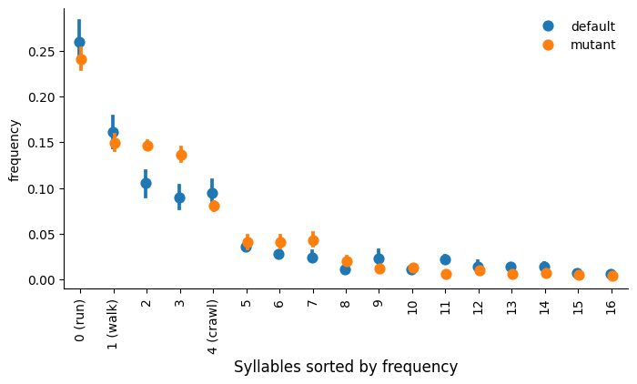
Test for statistically significant differences between groups of recordings. The code below takes a syllable property (e.g. frequency or duration), plots its disribution for each syllable across for each group, and also tests whether the property differs significantly between groups. The results are summarized in a plot that is saved to {project_dir}/{model_name}/analysis_figures.

There are two options for setting the order of syllables along the x-axis. When order='stat', syllables are sorted by the mean value of the statistic. When order='diff', syllables are sorted by the magnitude of difference between two groups that are determined by the ctrl_group and exp_group keywords. Note ctrl_group and exp_group are not related to significance testing.

kpms.plot_syll_stats_with_sem(
    stats_df, project_dir, model_name,
    plot_sig=True,    # whether to mark statistical significance with a star
    thresh=0.05,      # significance threshold
    stat='frequency', # statistic to be plotted (e.g. 'duration' or 'velocity_px_s_mean')
    order='stat',     # order syllables by overall frequency ("stat") or degree of difference ("diff")
    ctrl_group='a',   # name of the control group for statistical testing
    exp_group='b',    # name of the experimental group for statistical testing
    figsize=(8, 4),   # figure size    
    groups=stats_df['group'].unique(), # groups to be plotted
);

Saved figure to ../../testing/demo_project/2023_08_01-10_16_25/figures/frequency_stat_stats.png

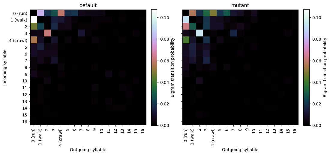
Transition matrices

Generate heatmaps showing the transition frequencies between syllables.

normalize='bigram' # normalization method ("bigram", "rows" or "columns")

trans_mats, usages, groups, syll_include=kpms.generate_transition_matrices(
    project_dir, model_name, normalize=normalize,
    min_frequency=0.005 # minimum syllable frequency to include
)    

kpms.visualize_transition_bigram(
    project_dir, model_name, groups, trans_mats, syll_include, normalize=normalize, 
    show_syllable_names=True # label syllables by index (False) or index and name (True)
)

Group(s): default, mutant
Saved figure to ../../testing/demo_project/2023_08_01-10_16_25/figures/transition_matrices.png

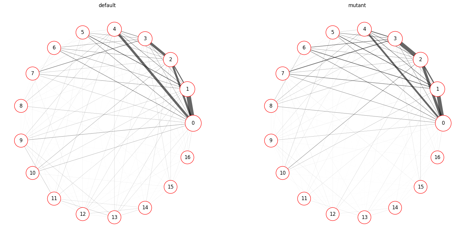
Syllable Transition Graph

Render transition rates in graph form, where nodes represent syllables and edges represent transitions between syllables, with edge width showing transition rate for each pair of syllables (secifically the max of the two transition rates in each direction).

# Generate a transition graph for each single group

kpms.plot_transition_graph_group(
    project_dir, model_name, 
    groups, trans_mats, usages, syll_include, 
    layout='circular',        # transition graph layout ("circular" or "spring")
    show_syllable_names=False # label syllables by index (False) or index and name (True)
)

Saved figure to ../../testing/demo_project/2023_08_01-10_16_25/figures/transition_graphs.png

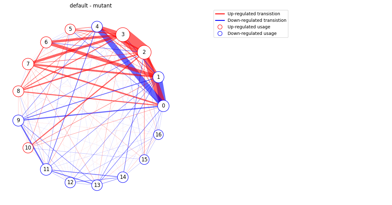
# Generate a difference-graph for each pair of groups.

kpms.plot_transition_graph_difference(project_dir, model_name, 
                                      groups, trans_mats, usages, syll_include, 
                                      layout='circular') # transition graph layout ("circular" or "spring")

Saved figure to ../../testing/demo_project/2023_08_01-10_16_25/figures/transition_graphs_diff.png