Exporting pose estimates
During fitting, keypoint-MoSeq tries to estimate the “true” pose trajectory of the animal, discounting anomolous or low-confidence keypoints. The pose trajectory is stored in the model as a variable “x” that encodes a low-dimensional representation of the keypoints (similar to PCA). The code below shows how to project the pose trajectory back into the original coordinate space. This is useful for visualizing the estimated pose trajectory.
import os
import h5py
import numpy as np
import jax.numpy as jnp
from jax_moseq.utils import unbatch
from jax_moseq.models.keypoint_slds import estimate_coordinates

# load the model (change project_dir and model_name as needed)
project_dir = 'demo_project'
model_name = '2023_08_01-10_16_25'
model, _, metadata, _ = kpms.load_checkpoint(project_dir, model_name)

# compute the estimated coordinates
Y_est = estimate_coordinates(
    jnp.array(model['states']['x']),
    jnp.array(model['states']['v']),
    jnp.array(model['states']['h']),
    jnp.array(model['params']['Cd'])
)

# generate a dictionary with reconstructed coordinates for each recording
coordinates_est = unbatch(Y_est, *metadata)
The following code generates a video showing frames 0-3600 from one recording with the reconstructed keypoints overlaid.
config = lambda: kpms.load_config(project_dir)
keypoint_data_path = 'dlc_project/videos' # can be a file, a directory, or a list of files
coordinates, confidences, bodyparts = kpms.load_keypoints(keypoint_data_path, 'deeplabcut')

recording_name = '21_11_8_one_mouse.top.irDLC_resnet50_moseq_exampleAug21shuffle1_500000'
video_path = 'dlc_project/videos/21_11_8_one_mouse.top.ir.mp4'

output_path = os.path.splitext(video_path)[0]+'.reconstructed_keypoints.mp4'
start_frame, end_frame = 0, 3600

kpms.overlay_keypoints_on_video(
    video_path,
    coordinates_est[recording_name],
    skeleton = config()['skeleton'],
    bodyparts = config()['use_bodyparts'],
    output_path = output_path,
    frames = range(start_frame, end_frame)
)
Automatic kappa scan
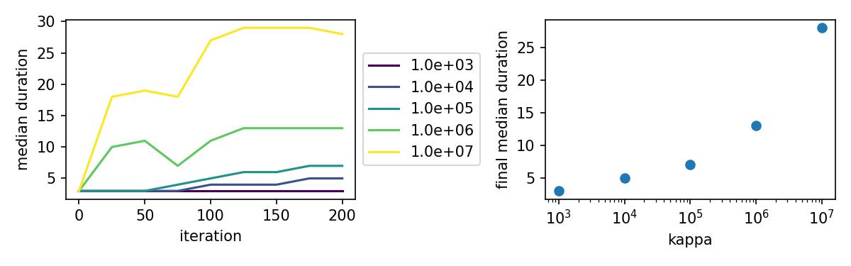
Keypoint-MoSeq includes a hyperparameter called kappa that determines the rate of transitions between syllables. Higher values of kappa lead to longer syllables and smaller values lead to shorter syllables. Users should choose a value of kappa based their desired distribution of syllable durations. The code below shows how to automatically scan over a range of kappa values and choose the optimal value.
Note
The following code reduces kappa by a factor of 10 (decrease_kappa_factor) before fitting the full model. You will need to recapitulate this step when fitting your own final model.
import numpy as np

kappas = np.logspace(3,7,5)
decrease_kappa_factor = 10
num_ar_iters = 50
num_full_iters = 200

prefix = 'my_kappa_scan'

for kappa in kappas:
    print(f"Fitting model with kappa={kappa}")
    model_name = f'{prefix}-{kappa}'
    model = kpms.init_model(data, pca=pca, **config())

    # stage 1: fit the model with AR only
    model = kpms.update_hypparams(model, kappa=kappa)
    model = kpms.fit_model(
        model,
        data,
        metadata,
        project_dir,
        model_name,
        ar_only=True,
        num_iters=num_ar_iters,
        save_every_n_iters=25
    )[0];

    # stage 2: fit the full model
    model = kpms.update_hypparams(model, kappa=kappa/decrease_kappa_factor)
    kpms.fit_model(
        model,
        data,
        metadata,
        project_dir,
        model_name,
        ar_only=False,
        start_iter=num_ar_iters,
        num_iters=num_full_iters,
        save_every_n_iters=25
    );

kpms.plot_kappa_scan(kappas, project_dir, prefix)
Model selection and comparison
Keypoint-MoSeq uses a stochastic fitting procedure, and thus produces slightly different syllable segmentations when run multiple times with different random seeds. Below, we show how to fit multiple models, compare the resulting syllables, and then select an optimal model for further analysis. It may also be useful in some cases to show that downstream analyses are robust to the choice of model.
Fitting multiple models
The code below shows how to fit multiple models with different random seeds.
import jax

num_model_fits = 20
prefix = 'my_models'

ar_only_kappa = 1e6
num_ar_iters = 50

full_model_kappa = 1e4
num_full_iters = 500

for restart in range(num_model_fits):
    print(f"Fitting model {restart}")
    model_name = f'{prefix}-{restart}'

    model = kpms.init_model(
        data, pca=pca, **config(), seed=jax.random.PRNGKey(restart)
    )

    # stage 1: fit the model with AR only
    model = kpms.update_hypparams(model, kappa=ar_only_kappa)
    model = kpms.fit_model(
        model,
        data,
        metadata,
        project_dir,
        model_name,
        ar_only=True,
        num_iters=num_ar_iters
    )[0]

    # stage 2: fit the full model
    model = kpms.update_hypparams(model, kappa=full_model_kappa)
    kpms.fit_model(
        model,
        data,
        metadata,
        project_dir,
        model_name,
        ar_only=False,
        start_iter=num_ar_iters,
        num_iters=num_full_iters
    );

    kpms.reindex_syllables_in_checkpoint(project_dir, model_name);
    model, data, metadata, current_iter = kpms.load_checkpoint(project_dir, model_name)
    results = kpms.extract_results(model, metadata, project_dir, model_name)
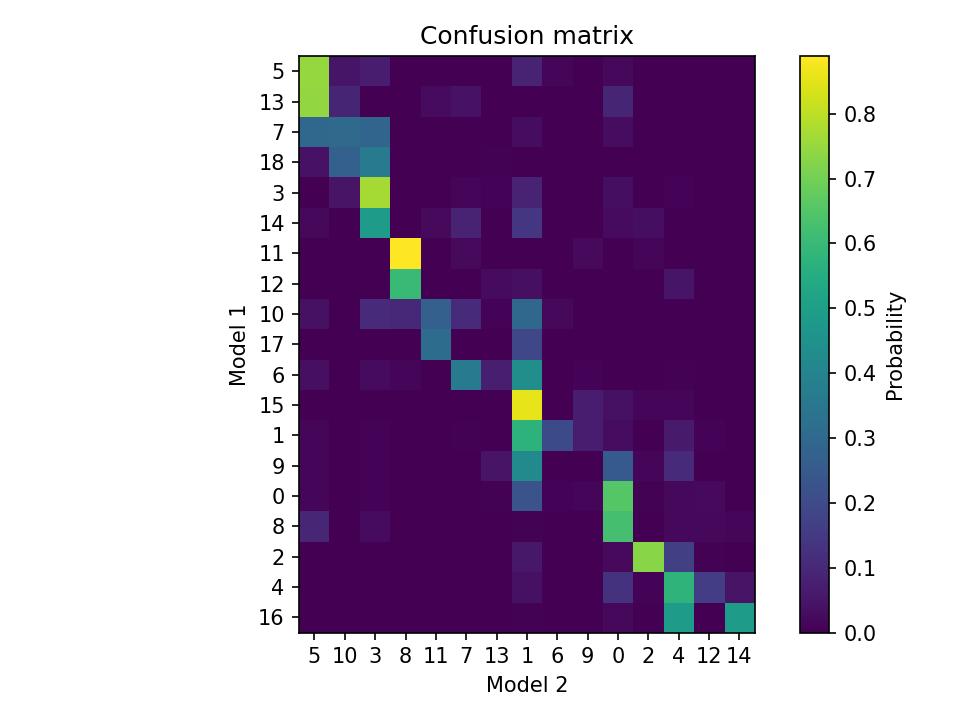
Comparing syllables
To get a sense of the variability across model runs, it may be useful to compare syllables produced by each model. The code below shows how to load results from two models runs (e.g., produced by the code above) and plot a confusion matrix showing the overlap between syllable labels.
model_name_1 = 'my_models-0'
model_name_2 = 'my_models-1'

results_1 = kpms.load_results(project_dir, model_name_1)
results_2 = kpms.load_results(project_dir, model_name_2)

kpms.plot_confusion_matrix(results_1, results_2);
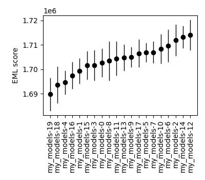
Selecting a model
We developed a matric called the expected marginal likelihood (EML) score that can be used to rank models. To calculate EML scores, you must first fit an ensemble of models to a given dataset, as shown in Fitting multiple models. The code below loads this ensemble and then calculates the EML score for each model. The model with the highest EML score can then be selected for further analysis.
# change the following line as needed
model_names = ['my_models-{}'.format(i) for i in range(20)]

eml_scores, eml_std_errs = kpms.expected_marginal_likelihoods(project_dir, model_names)
best_model = model_names[np.argmax(eml_scores)]
print(f"Best model: {best_model_name}")

kpms.plot_eml_scores(eml_scores, eml_std_errs, model_names)
Model averaging
Keypoint-MoSeq is probabilistic. So even once fitting is complete and the syllable parameters are fixed, there is still a distribution of possible syllable sequences given the observed data. In the default pipeline, one such sequence is sampled from this distribution and used for downstream analyses. Alternatively, one can estimate the marginal probability distribution over syllable labels at each timepoint. The code below shows how to do this. It can be applied to new data or the same data that was used for fitting (or a combination of the two).
burnin_iters = 200
num_samples = 100
steps_per_sample = 5

# load the model (change `project_dir` and `model_name` as needed)
model = kpms.load_checkpoint(project_dir, model_name)[0]

# load data (e.g. from deeplabcut)
data_path = 'path/to/data/' # can be a file, a directory, or a list of files
coordinates, confidences, bodyparts = kpms.load_keypoints(data_path, 'deeplabcut')
data, metadata = kpms.format_data(coordinates, confidences, **config())

# compute the marginal probabilities of syllable labels
marginal_probs = kpms.estimate_syllable_marginals(
    model, data, metadata, burnin_iters, num_samples, steps_per_sample, **config()
)
Location-aware modeling
Because keypoint-MoSeq uses centered and aligned pose estimates to define syllables, it is effectively blind to absolute movements of the animal in space. The only thing that keypoint-MoSeq normally cares about is change in pose – defined here as the relative location of each keypoint. For example, if an animal were capable of simply sliding forward without otherwise moving, this would fail to show up in the syllable segmentation. To address this gap, we developed an experimental version of keypoint-MoSeq that leverages location and heading dynamics (in addition to pose) when defining syllables. To use this “location-aware” model, simply pass location_aware=True as an additional argument when calling the following functions.
keypoint_moseq.init_model()keypoint_moseq.fit_model()keypoint_moseq.apply_model()keypoint_moseq.estimate_syllable_marginals()
Note that the location-aware model was not tested in the keypoint-MoSeq paper remains experimental. We welcome feedback and suggestions for improvement.
Mathematical details
In the published version of keypoint-MoSeq, the animal’s location \(v_t\) and heading \(h_t\) at each timepoint are conditionally independent of the current syllable \(z_t\). In particular, we assume
In the location-aware model, we relax this assumption and allow the animal’s location and heading to depend on the current syllable. Specifically, each syllable is associated with a pair of normal distributions that specify the animal’s expected rotation and translation at each timestep. This can be expressed formally as follows:
where \(R(h)\) is a rotation matrix that rotates a vector by angle \(h\). The parameters \(\Delta h_i\), \(\Delta v_i\), \(\sigma^2_{h,i}\), and \(\sigma^2_{v,i}\) for each syllable \(i\) have a normal-inverse-gamma prior:
Temporal downsampling
Sometimes it’s useful to downsample a dataset, e.g. if the original recording has a much higher framerate than is needed for modeling. To downsample, run the following lines right after loading the keypoints.
downsample_rate = 2 # keep every 2nd frame
coordinates, video_frame_indexes = kpms.downsample_timepoints(
    coordinates, downsample_rate
)
confidences, video_frame_indexes = kpms.downsample_timepoints(
    confidences, downsample_rate
) # skip if `confidences=None`
After this, the pipeline can be run as usual, except for steps that involve reading the original videos, in which case video_frame_indexes should be passed as an additional argument.
# Calibration step
kpms.noise_calibration(..., video_frame_indexes=video_frame_indexes)

# Making grid movies
kpms.generate_grid_movies(..., video_frame_indexes=video_frame_indexes)

# Overlaying keypoints
kpms.overlay_keypoints_on_video(..., video_frame_indexes=video_frame_indexes)
Trimming inputs
In some datasets, the animal is missing at the beginning and/or end of each video. In these cases, the easiest solution is to trim the videos before running keypoint detection. However, it’s also possible to directly trim the inputs to keypoint-MoSeq. Let’s assume that you already have a dictionary called bounds that has the same keys as coordinates and contains the desired start/end times for each recording. The next step would be to trim coordinates and confindences
coordinates = {k: coords[bounds[k][0]:bounds[k][1]] for k,coords in coordinates.items()}
confidences = {k: confs[bounds[k][0]:bounds[k][1]] for k,confs in confidences.items()}
You’ll also need to generate a dictionary called video_frame_indexes that maps the timepoints of coordinates and confindences to frame indexes from the original videos.
import numpy as np
video_frame_indexes = {k : np.arange(bounds[k][0], bounds[k][1]) for k in bounds}
After this, the pipeline can be run as usual, except for steps that involve reading the original videos, in which case video_frame_indexes should be passed as an additional argument.
# Calibration step
kpms.noise_calibration(..., video_frame_indexes=video_frame_indexes)

# Making grid movies
kpms.generate_grid_movies(..., video_frame_indexes=video_frame_indexes)

# Overlaying keypoints
kpms.overlay_keypoints_on_video(..., video_frame_indexes=video_frame_indexes)
Merging similar syllables
In some cases it may be convenient to combine syllables that represent similar behaviors. Keypoint-moseq provides convenience functions for merging syllables into user-defined groups. These groups could be based on inspection of trajecotry plots, grid movies, or syllable dendrograms.
# Define the syllables to merge as a list of lists. All syllables within
# a given inner list will be merged into a single syllable.
# In this case, we're merging syllables 1 and 3 into a single syllable,
# and merging syllables 4 and 5 into a single syllable.
syllables_to_merge = [
    [1, 3],
    [4, 5]
]

# Load the results you wish to merge (change path as needed)
import os
results_path = os.path.join(project_dir, model_name, 'results.h5')
results = kpms.load_hdf5(results_path)

# Generate a mapping that specifies how syllables will be relabled.
syllable_mapping = kpms.generate_syllable_mapping(results, syllables_to_merge)
new_results = kpms.apply_syllable_mapping(results, syllable_mapping)

# Save the new results to disk (using a modified path)
new_results_path = os.path.join(project_dir, model_name, 'results_merged.h5')
kpms.save_hdf5(new_results_path, new_results)

# Optionally generate new trajectory plots and grid movies
# In each case, specify the output directory to avoid overwriting
output_dir = os.path.join(project_dir, model_name, 'grid_movies_merged')
kpms.generate_grid_movies(new_results, output_dir=output_dir, coordinates=coordinates, **config())

output_dir = os.path.join(project_dir, model_name, 'trajectory_plots_merged')
kpms.generate_trajectory_plots(coordinates, new_results, output_dir=output_dir, **config())