This notebook shows how to setup a new project, train a keypoint-MoSeq model and visualize the resulting syllables.
Note
To ensure prevent errors during the calibration step below, make sure to launch jupyter from the keypoint_moseq environment.
Project setup
Create a new project directory with a keypoint-MoSeq config.yml file.
import keypoint_moseq as kpms
import matplotlib.pyplot as plt
project_dir = "demo_project"
config = lambda: kpms.load_config(project_dir)
Edit the config file
The config can be edited in a text editor or using the function kpms.update_config, as shown below. In general, the following parameters should be specified for each project:
bodyparts(name of each keypoint; automatically imported from SLEAP/DeepLabCut)use_bodyparts(subset of bodyparts to use for modeling, set to all bodyparts by default; for mice we recommend excluding the tail)anterior_bodypartsandposterior_bodyparts(used for rotational alignment)video_dir(directory with videos of each experiment)fps(frame per second of the input video)
Edit the config as follows for the example DeepLabCut dataset:
kpms.update_config(
project_dir,
video_dir="dlc_project/videos/",
anterior_bodyparts=["nose"],
posterior_bodyparts=["spine4"],
use_bodyparts=["spine4", "spine3", "spine2", "spine1", "head", "nose", "right ear", "left ear"],
fps=30,
)
Load data
The code below shows how to load keypoint detections from DeepLabCut. To load other formats, replace 'deeplabcut' in the example with one of 'sleap', 'anipose', 'sleap-anipose', 'nwb'. For other formats, see the FAQ.
# load data (e.g. from DeepLabCut)
keypoint_data_path = "dlc_project/videos/" # can be a file, a directory, or a list of files
coordinates, confidences, bodyparts = kpms.load_keypoints(keypoint_data_path, "deeplabcut")
Remove outlier keypoints
Removing large outliers can improve the robustness of model fitting. A common type of outlier is a keypoint which briefly moves very far away from the animal as the result of a tracking error. The following cell classifies keypoints as outliers based on their distance to the animal’s medoid. The outlier keypoints are then interpolated and their confidences are set to 0 so that they are interpolated for modeling as well.
Use
outlier_scale_factorto adjust the stringency of outlier detection (higher values -> more stringent)Plots showing distance to medoid before and after outlier interpolation are saved to
{project_dir}/QA/plots/Plotting can take a few minutes, so by default plots will not be regenerated when re-running this cell. To experiment with the effects of setting different values for outlier_scale_factor, set
overwrite=Truein outlier_removal.
kpms.update_config(project_dir, outlier_scale_factor=6.0)
coordinates, confidences = kpms.outlier_removal(
coordinates,
confidences,
project_dir,
overwrite=False,
**config()
)
Format data for modeling
data, metadata = kpms.format_data(coordinates, confidences, **config())
Calibration
The purpose of calibration is to learn the relationship between keypoint errors and confidence scores. The results are stored using the slope and intercept parameters in the config.
Run the cell below. A widget should appear with a video frame and the name of a bodypart. A yellow marker denotes the detected location of the bodypart.
Annotate each frame with the correct location of the labeled bodypart
Click on the image at the correct location - an “X” should appear.
Use the prev/next buttons to annotate additional frames.
Click and drag the bottom-right shaded corner of the widget to adjust image size.
Use the toolbar to the left of the figure to pan and zoom.
We suggest annotating at least 50 frames.
Annotations will be automatically saved once you’ve completed at least 20 annotations. Each new annotation after that will trigger an auto-save of all your work. The message at the top of the widget will indicate when your annotations are being saved.
%matplotlib widget
kpms.noise_calibration(project_dir, coordinates, confidences, **config())
Loading sample frames: 100%|████████████| 90/90 [00:06<00:00, 14.25it/s]


WARNING:param.OverlayPlot01356: Tool of type 'pan' could not be found and could not be activated by default.
WARNING:param.OverlayPlot01356:Tool of type 'pan' could not be found and could not be activated by default.
WARNING:param.OverlayPlot01356: Tool of type 'wheel_zoom' could not be found and could not be activated by default.
WARNING:param.OverlayPlot01356:Tool of type 'wheel_zoom' could not be found and could not be activated by default.
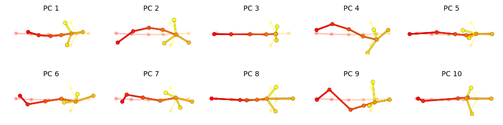
Fit PCA
Run the cell below to fit a PCA model to aligned and centered keypoint coordinates.
The model is saved to
{project_dir}/pca.pand can be reloaded usingkpms.load_pca.Two plots are generated: a cumulative scree plot and a depiction of each PC, where translucent nodes/edges represent the mean pose and opaque nodes/edges represent a perturbation in the direction of the PC.
After fitting, edit
latent_dimensionin the config. This determines the dimension of the pose trajectory used to fit keypoint-MoSeq. A good heuristic is the number of dimensions needed to explain 90% of variance, or 10 dimensions - whichever is lower.
plt.close("all")
%matplotlib inline
pca = kpms.fit_pca(**data, **config())
kpms.save_pca(pca, project_dir)
kpms.print_dims_to_explain_variance(pca, 0.9)
kpms.plot_scree(pca, project_dir=project_dir)
kpms.plot_pcs(pca, project_dir=project_dir, **config())
# use the following to load an already fit model
# pca = kpms.load_pca(project_dir)
>=90.0% of variance exlained by 4 components.
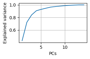
kpms.update_config(project_dir, latent_dim=4)
Model fitting
Fitting a keypoint-MoSeq model involves:
Estimating hyperparameters: Set model hyperparameters that can be automatically estimated from the input data.
Initialization: Auto-regressive (AR) parameters and syllable sequences are randomly initialized using pose trajectories from PCA.
Fitting an AR-HMM: The AR parameters, transition probabilities and syllable sequences are iteratively updated through Gibbs sampling.
Fitting the full model: All parameters, including both the AR-HMM as well as centroid, heading, noise-estimates and continuous latent states (i.e. pose trajectories) are iteratively updated through Gibbs sampling. This step is especially useful for noisy data.
Extracting model results: The learned states of the model are parsed and saved to disk for vizualization and downstream analysis.
[Optional] Applying the trained model: The learned model parameters can be used to infer a syllable sequences for additional data.
Setting kappa
Most users will need to adjust the kappa hyperparameter to achieve the desired distribution of syllable durations. For this tutorial we chose kappa values that yielded a median syllable duration of 400ms (12 frames). Most users will need to tune kappa to their particular dataset. Higher values of kappa lead to longer syllables. You will need to pick two kappas: one for AR-HMM fitting and one for the full model.
We recommend iteratively updating kappa and refitting the model until the target syllable time-scale is attained.
Model fitting can be stopped at any time by interrupting the kernel, and then restarted with a new kappa value.
The full model will generally require a lower value of kappa to yield the same target syllable durations.
To adjust the value of kappa in the model, use
kpms.update_hypparamsas shown below. Note that this command only changes kappa in the model dictionary, not the kappa value in the config file. The value in the config is only used during model initialization.
Estimating Hyperparameters
We provide heuristics for adjusting a subset of model hyperparameters:
sigmasq_loc: The expected distance that the centroid will move each frame. If this is set too high, the centroid trajectory will be overly noisy. If it’s set too low, the centroid may deviate from the animal’s true location during fast locomotion.
estimate_sigmasq_locestimates this hyperparameter based on the empirical frame-to-frame movement of the filtered centroid trajectory.
kpms.update_config(
project_dir,
sigmasq_loc=kpms.estimate_sigmasq_loc(data["Y"], data["mask"], filter_size=config()["fps"])
)
Initialization
# initialize the model
model = kpms.init_model(data, pca=pca, **config())
# optionally modify kappa
# model = kpms.update_hypparams(model, kappa=NUMBER)
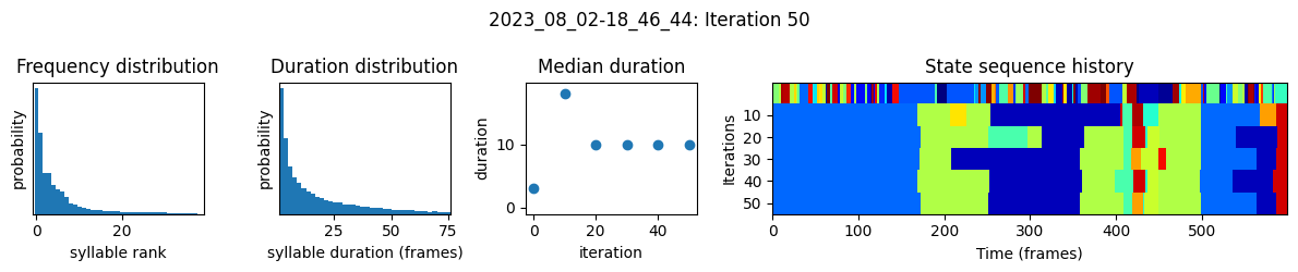
Fitting an AR-HMM
In addition to fitting an AR-HMM, the function below:
generates a name for the model and a corresponding directory in
project_dirsaves a checkpoint every 25 iterations from which fitting can be restarted
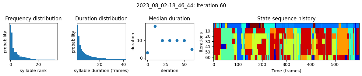
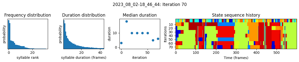
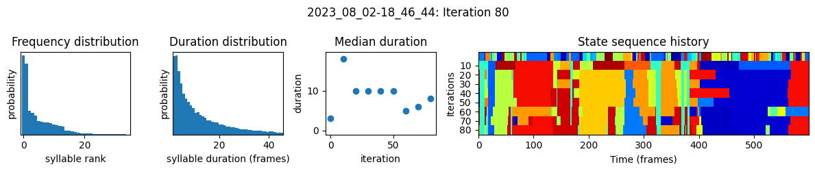
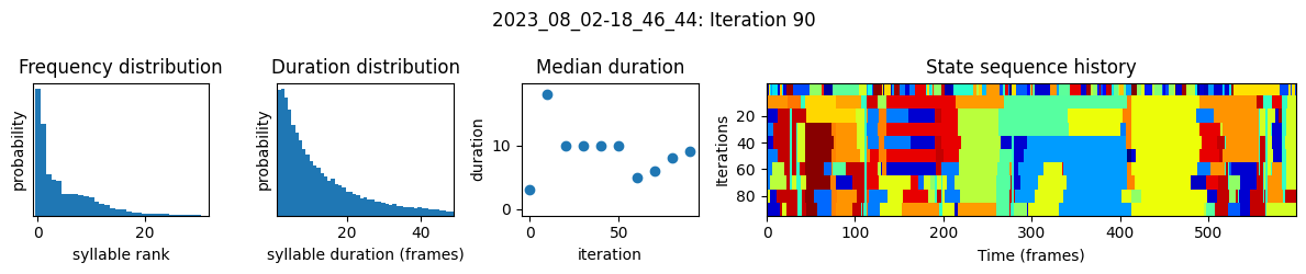
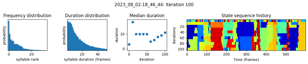
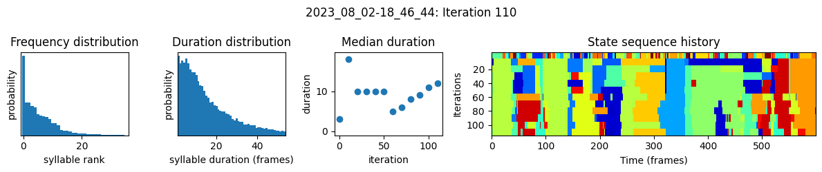
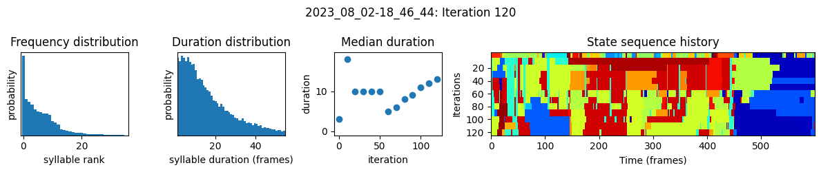
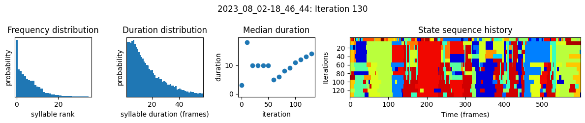
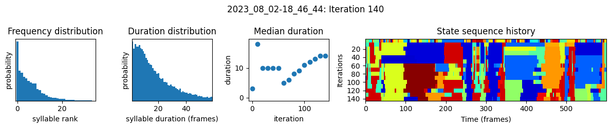
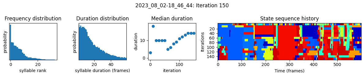
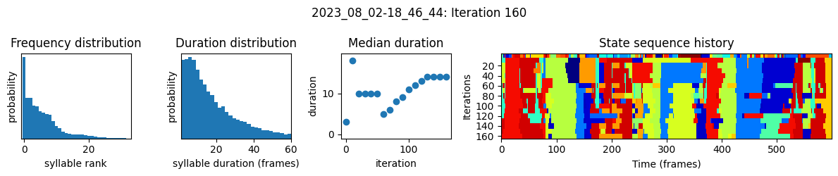
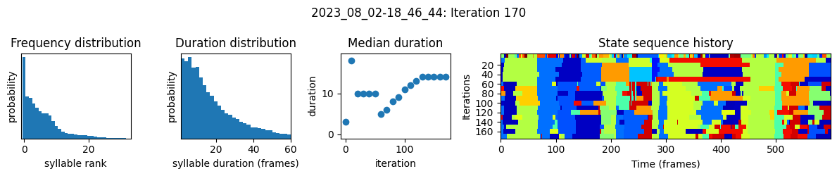
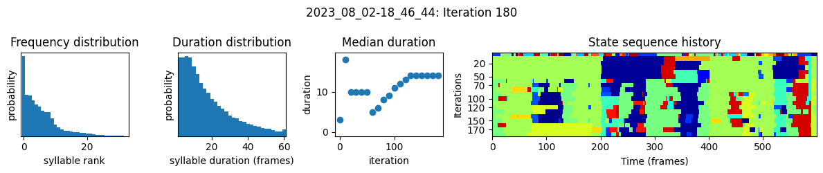
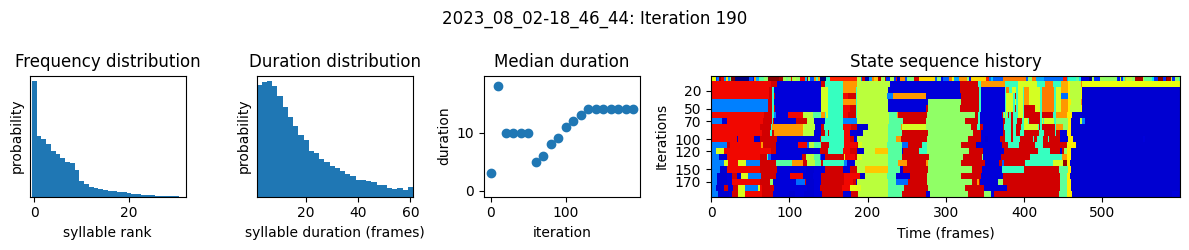
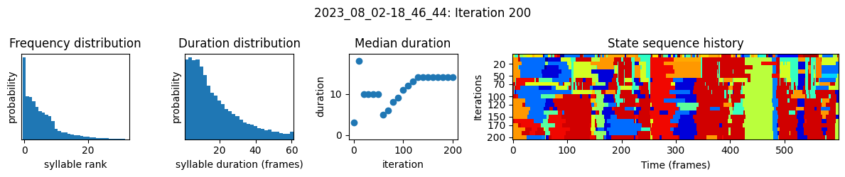
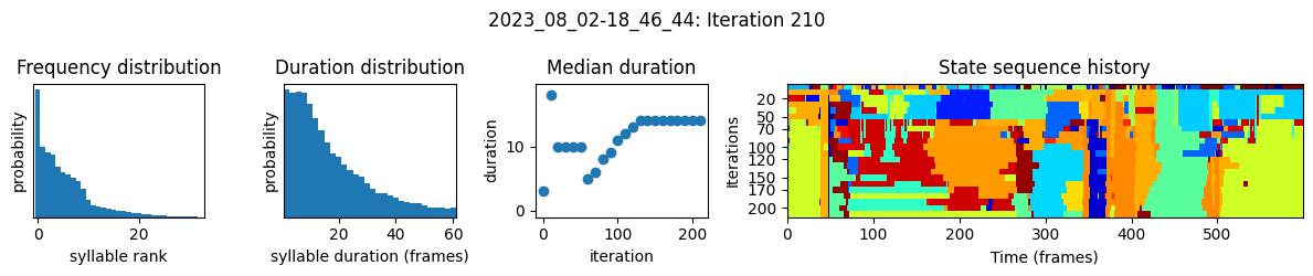
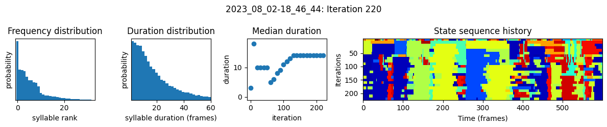
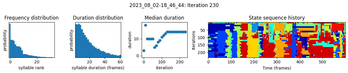
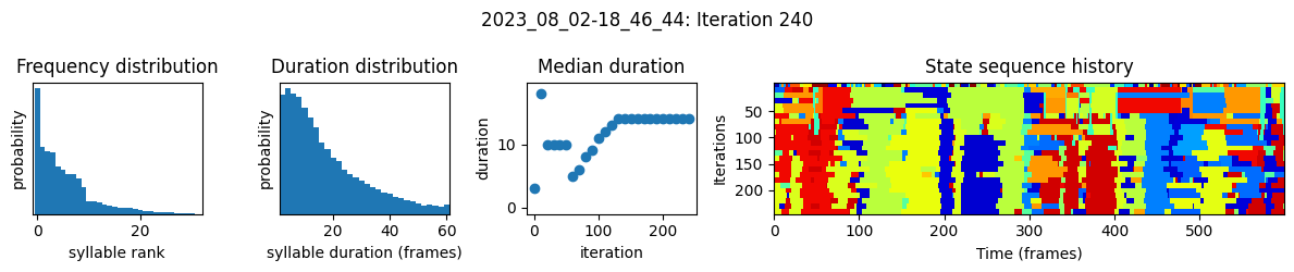
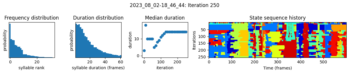
plots the progress of fitting every 25 iterations, including
the distributions of syllable frequencies and durations for the most recent iteration
the change in median syllable duration across fitting iterations
a sample of the syllable sequence across iterations in a random window
Note: Some users have reported systematic differences in the way syllables are assigned when applying a model to new data. To control for this, we recommend running apply_model to both the new and original data and using these new results instead of the original model output. To save the original results, simply rename the original results.h5 file or save the new results to a different filename using results_path="new_file_name.h5".
num_ar_iters = 50
model, model_name = kpms.fit_model(
model, data, metadata, project_dir, ar_only=True, num_iters=num_ar_iters
)
Outputs will be saved to demo_project/2023_08_02-18_46_44
20%|██████▊ | 10/51 [00:25<01:19, 1.93s/it]
100%|███████████████████████████████████| 51/51 [02:03<00:00, 2.42s/it]
Fitting the full model
The following code fits a full keypoint-MoSeq model using the results of AR-HMM fitting for initialization. If using your own data, you may need to try a few values of kappa at this step.
# load model checkpoint
model, data, metadata, current_iter = kpms.load_checkpoint(
project_dir, model_name, iteration=num_ar_iters
)
# modify kappa to maintain the desired syllable time-scale
model = kpms.update_hypparams(model, kappa=1e4)
# run fitting for an additional 500 iters
model = kpms.fit_model(
model,
data,
metadata,
project_dir,
model_name,
ar_only=False,
start_iter=current_iter,
num_iters=current_iter + 500,
)[0]
Outputs will be saved to demo_project/2023_08_02-18_46_44
5%|█▋ | 10/201 [01:44<12:01, 3.78s/it]
10%|███▍ | 20/201 [02:15<08:42, 2.88s/it]
15%|█████ | 30/201 [02:46<08:10, 2.87s/it]
20%|██████▊ | 40/201 [03:18<07:44, 2.88s/it]
25%|████████▍ | 50/201 [03:49<07:12, 2.86s/it]
30%|██████████▏ | 60/201 [04:30<06:59, 2.98s/it]
35%|███████████▊ | 70/201 [05:01<06:16, 2.88s/it]
40%|█████████████▌ | 80/201 [05:34<05:48, 2.88s/it]
45%|███████████████▏ | 90/201 [06:05<05:18, 2.87s/it]
50%|████████████████▍ | 100/201 [06:37<04:49, 2.87s/it]
55%|██████████████████ | 110/201 [07:08<04:20, 2.86s/it]
60%|███████████████████▋ | 120/201 [07:48<04:01, 2.98s/it]
65%|█████████████████████▎ | 130/201 [08:20<03:24, 2.89s/it]
70%|██████████████████████▉ | 140/201 [08:51<02:54, 2.86s/it]
75%|████████████████████████▋ | 150/201 [09:33<02:32, 3.00s/it]
80%|██████████████████████████▎ | 160/201 [10:04<01:57, 2.87s/it]
85%|███████████████████████████▉ | 170/201 [10:45<01:32, 2.97s/it]
90%|█████████████████████████████▌ | 180/201 [11:16<01:00, 2.87s/it]
95%|███████████████████████████████▏ | 190/201 [11:47<00:31, 2.88s/it]
100%|████████████████████████████████▊| 200/201 [12:19<00:02, 2.87s/it]
100%|█████████████████████████████████| 201/201 [12:25<00:00, 3.71s/it]
Sort syllables by frequency
Permute the states and parameters of a saved checkpoint so that syllables are labeled in order of frequency (i.e. so that 0 is the most frequent, 1 is the second most, and so on).
# modify a saved checkpoint so syllables are ordered by frequency
kpms.reindex_syllables_in_checkpoint(project_dir, model_name);
Reindexing: 100%|███████████| 26/26 [01:15<00:00, 2.90s/model snapshot]
Warning
Reindexing is only applied to the checkpoint file. Therefore, if you perform this step after extracting the modeling results or generating vizualizations, then those steps must be repeated.
Extract model results
Parse the modeling results and save them to {project_dir}/{model_name}/results.h5. The results are stored as follows, and can be reloaded at a later time using kpms.load_results. Check the docs for an in-depth explanation of the modeling results.
results.h5
├──recording_name1
│ ├──syllable # syllable labels (z)
│ ├──latent_state # inferred low-dim pose state (x)
│ ├──centroid # inferred centroid (v)
│ └──heading # inferred heading (h)
⋮
# load the most recent model checkpoint
model, data, metadata, current_iter = kpms.load_checkpoint(project_dir, model_name)
# extract results
results = kpms.extract_results(model, metadata, project_dir, model_name)
Saved results to demo_project/2023_08_02-18_46_44/results.h5
[Optional] Save results to csv
After extracting to an h5 file, the results can also be saved as csv files. A separate file will be created for each recording and saved to {project_dir}/{model_name}/results/.
# optionally save results as csv
kpms.save_results_as_csv(results, project_dir, model_name)
Saving to csv: 100%|████████████████████| 10/10 [00:04<00:00, 2.46it/s]
Apply to new data
The code below shows how to apply a trained model to new data. This is useful if you have performed new experiments and would like to maintain an existing set of syllables. The results for the new experiments will be added to the existing results.h5 file. This step is optional and can be skipped if you do not have new data to add.
# load the most recent model checkpoint and pca object
model = kpms.load_checkpoint(project_dir, model_name)[0]
# load new data (e.g. from deeplabcut)
new_data = "path/to/new/data/" # can be a file, a directory, or a list of files
coordinates, confidences, bodyparts = kpms.load_keypoints(new_data, "deeplabcut")
coordinates, confidences = kpms.outlier_removal(
coordinates,
confidences,
project_dir,
overwrite=False,
**config()
)
data, metadata = kpms.format_data(coordinates, confidences, **config())
# apply saved model to new data
results = kpms.apply_model(model, data, metadata, project_dir, model_name, **config())
# optionally rerun `save_results_as_csv` to export the new results
# kpms.save_results_as_csv(results, project_dir, model_name)
Visualization
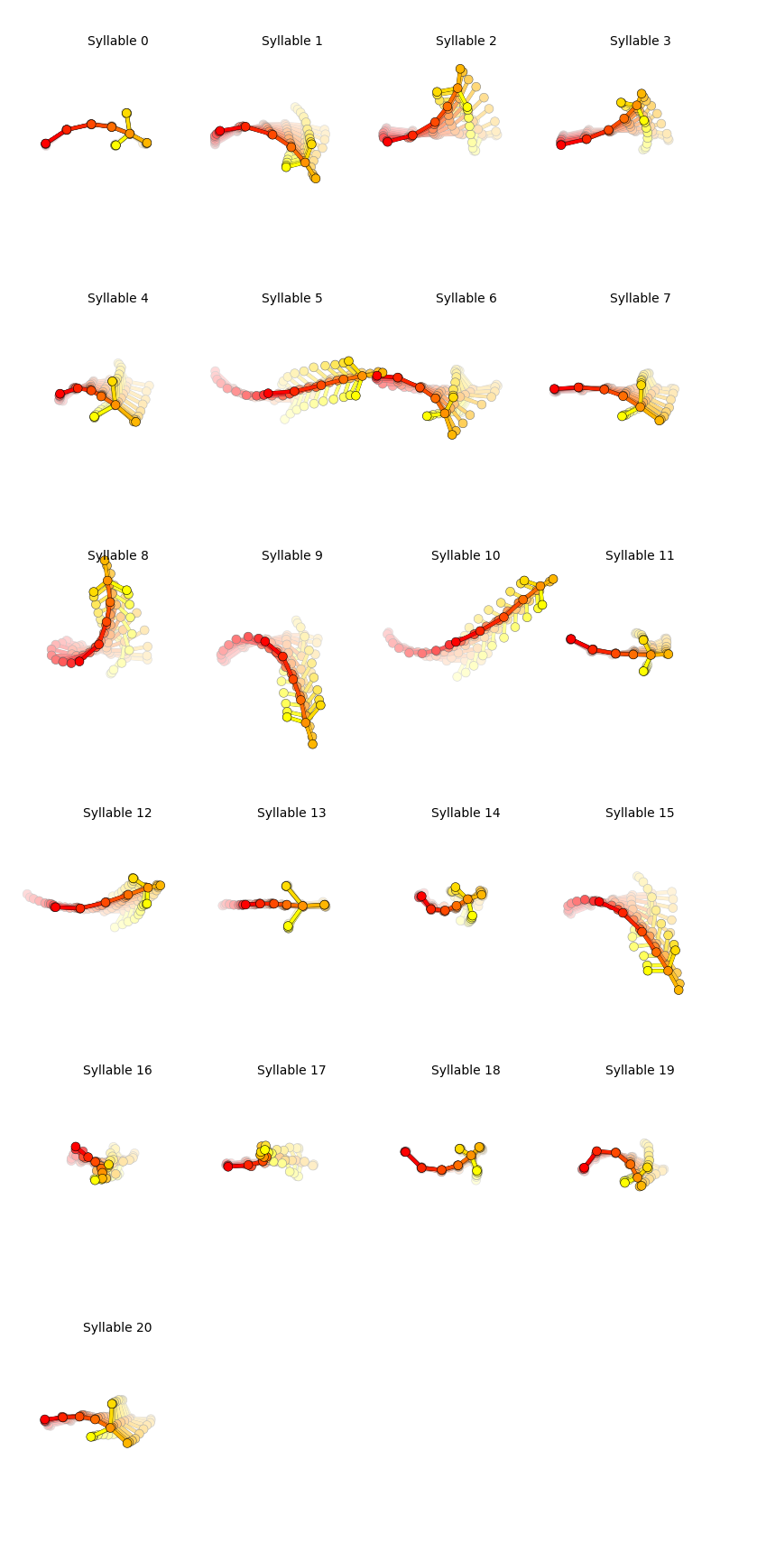
Trajectory plots
Generate plots showing the median trajectory of poses associated with each given syllable.
results = kpms.load_results(project_dir, model_name)
kpms.generate_trajectory_plots(coordinates, results, project_dir, model_name, **config())
Saving trajectory plots to demo_project/2023_08_02-18_46_44/grid_movies
Generating trajectory plots: 100%|██████| 21/21 [00:09<00:00, 2.31it/s]
Grid movies
Generate video clips showing examples of each syllable.
Note: the code below will only work with 2D data. For 3D data, see the FAQ.
kpms.generate_grid_movies(results, project_dir, model_name, coordinates=coordinates, **config());
Writing grid movies to demo_project/2023_08_02-18_46_44/grid_movies
Generating grid movies: 100%|███████████| 21/21 [02:04<00:00, 5.91s/it]
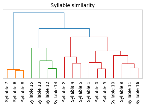
Syllable Dendrogram
Plot a dendrogram representing distances between each syllable’s median trajectory.
kpms.plot_similarity_dendrogram(coordinates, results, project_dir, model_name, **config())
Saving dendrogram plot to ../../testing/demo_project/2023_08_01-10_16_25/similarity_dendrogram